Recursion (computer science)
| Programming paradigms |
|---|
|
Recursion in computer science is a method where the solution to a problem depends on solutions to smaller instances of the same problem.[1] The approach can be applied to many types of problems, and is one of the central ideas of computer science.[2]
"The power of recursion evidently lies in the possibility of defining an infinite set of objects by a finite statement. In the same manner, an infinite number of computations can be described by a finite recursive program, even if this program contains no explicit repetitions." [3]
Most computer programming languages support recursion by allowing a function to call itself within the program text. Some functional programming languages do not define any looping constructs but rely solely on recursion to repeatedly call code. Computability theory has proven that these recursive-only languages are mathematically equivalent to the imperative languages, meaning they can solve the same kinds of problems even without the typical control structures like “while” and “for”.
Contents |
Recursive data types
Many computer programs must process or generate an arbitrarily large quantity of data. Recursion is one technique for representing data whose exact size the programmer does not know: the programmer can specify this data with a self-referential definition. There are two types of self-referential definitions: inductive and coinductive definitions.
Inductively-defined data
An inductively-defined recursive data definition is one that specifies how to construct instances of the data. For example, linked lists can be defined inductively (here, using Haskell syntax):
data ListOfStrings = EmptyList | Cons String ListOfStrings
The code above specifies a list of strings to be either empty, or a structure that contains a string and a list of strings. The self-reference in the definition permits the construction of lists of any (finite) number of strings.
Another example of inductive definition is the natural numbers (or non-negative integers):
A natural number is either 1 or n+1, where n is a natural number.
Similarly recursive definitions are often used to model the structure of expressions and statements in programming languages. Language designers often express grammars in a syntax such as Backus-Naur form; here is such a grammar, for a simple language of arithmetic expressions with multiplication and addition:
 <expr> ::= <number>
          | (<expr> * <expr>)
          | (<expr> + <expr>)
This says that an expression is either a number, a product of two expressions, or a sum of two expressions. By recursively referring to expressions in the second and third lines, the grammar permits arbitrarily complex arithmetic expressions such as (5 * ((3 * 6) + 8)), with more than one product or sum operation in a single expression.
Coinductively-defined data and corecursion
A coinductive data definition is one that specifies the operations that may be performed on a piece of data; typically, self-referential coinductive definitions are used for data structures of infinite size.
A coinductive definition of infinite streams of strings, given informally, might look like this:
A stream of strings is an object s such that
 head(s) is a string, and
 tail(s) is a stream of strings.
This is very similar to an inductive definition of lists of strings; the difference is that this definition specifies how to access the contents of the data structure—namely, via the accessor functions head and tail -- and what those contents may be, whereas the inductive definition specifies how to create the structure and what it may be created from.
Corecursion is related to coinduction, and can be used to compute particular instances of (possibly) infinite objects. As a programming technique, it is used most often in the context of lazy programming languages, and can be preferable to recursion when the desired size or precision of a program's output is unknown. In such cases the program requires both a definition for an infinitely large (or infinitely precise) result, and a mechanism for taking a finite portion of that result. The problem of computing the first n prime numbers is one that can be solved with a corecursive program.
Structural versus generative recursion
Some authors classify recursion as either "generative" or "structural". The distinction is related to where a recursive procedure gets the data that it works on, and how it processes that data: proving termination of a function. All structurally-recursive functions on finite (inductively-defined) data structures can easily be shown to terminate, via structural induction: intuitively, each recursive call receives a smaller piece of input data, until a base case is reached. Generatively-recursive functions, in contrast, do not necessarily feed smaller input to their recursive calls, so proof of their termination is not necessarily as simple, and avoiding infinite loops requires greater care.
Recursive programs
Recursive procedures
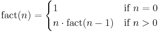
Factorial
A classic example of a recursive procedure is the function used to calculate the factorial of a natural number:
| Pseudocode (recursive): |
|---|
function factorial is: |
The function can also be written as a recurrence relation:


This evaluation of the recurrence relation demonstrates the computation that would be performed in evaluating the pseudocode above:
| Computing the recurrence relation for n = 4: |
|---|
b4 = 4 * b3 |
This factorial function can also be described without using recursion by making use of the typical looping constructs found in imperative programming languages:
| Pseudocode (iterative): |
|---|
function factorial is: |
The imperative code above is equivalent to this mathematical definition using an accumulator variable t:
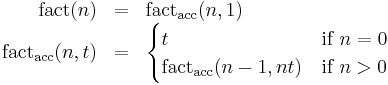
The definition above translates straightforwardly to functional programming languages such as Scheme; this is an example of iteration implemented recursively.
Fibonacci
Another well known mathematical recursive function is one that computes the Fibonacci numbers: 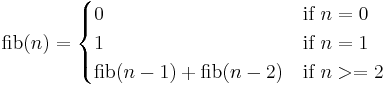
| Pseudocode |
|---|
function fib is: input: integer n such that n >= 0 |
Java language implementation:
    /**
     * Recursively calculate the kth Fibonacci number.
     *
     * @param k indicates which (positive) Fibonacci number to compute.
     * @return the kth Fibonacci number.
     */
    private static int fib(int k) {

	// Base Cases:
        //   If k == 0 then fib(k) = 0.
	//   If k == 1 then fib(k) = 1.
	if (k < 2) {
            return k;
	}
	// Recursive Case:
	//   If k >= 2 then fib(k) = fib(k-1) + fib(k-2).
	else {
	    return fib(k-1) + fib(k-2);
	}
    }
Python language implementation:
def fib(n):
    if n < 2:
        return n
    else:
        return fib(n-1) + fib(n-2)
Scheme language implementation:
JavaScript language implementation:
function fib (n) {
    if (!n) {
        return 0;
    } else if (n <= 2) {
        return 1;
    } else {
        return fib(n - 1) + fib(n - 2);
    }
}
Common Lisp implementation:
(defun fib (n)
  (cond ((= n 0) 0)
        ((= n 1) 1)
        (t (+ (fib (- n 1))
              (fib (- n 2))))))
Recurrence relation for Fibonacci:
bn = bn-1 + bn-2
b1 = 1, b0 = 0
| Computing the recurrence relation for n = 4: |
|---|
  b4            = b3 + b2
                = b2 + b1 + b1 + b0
                = b1 + b0 + 1 + 1 + 0
                = 1 + 0 + 1 + 1 + 0
                = 3
|
This Fibonacci algorithm is a particularly poor example of recursion, because each time the function is executed on a number greater than one, it makes two function calls to itself, leading to an exponential number of calls (and thus exponential time complexity) in total.[4] The following alternative approach uses two accumulator variables TwoBack and OneBack to "remember" the previous two Fibonacci numbers constructed, and so avoids the exponential time cost:
| Pseudocode |
|---|
function fib is:
input: integer Times such that Times >= 0, relative to TwoBack and OneBack
long TwoBack such that TwoBack = fib(x)
long OneBack such that OneBack = fib(x)
|
To obtain the tenth number in the Fib. sequence, one must perform Fib(10,0,1). Where 0 is considered TwoNumbers back and 1 is considered OneNumber back. As can be seen in this approach, no trees are being created, therefore the efficiency is much greater, being a linear recursion. The recursion in condition 4, shows that OneNumber back becomes TwoNumbers back, and the new OneNumber back is calculated, simply decrementing the Times on each recursion.
Implemented in the Java or the C# programming language:
public static long fibonacciOf(int times, long twoNumbersBack, long oneNumberBack) {

    if (times == 0) {                            // Used only for fibonacciOf(0, 0, 1)
        return twoNumbersBack;
    } else if (times == 1) {                     // Used only for fibonacciOf(1, 0, 1)
        return oneNumberBack;
    } else if (times == 2) {                     // When the 0 and 1 clauses are included,
        return oneNumberBack + twoNumbersBack;   // this clause merely stops one additional
    } else {                                     // recursion from occurring
        return fibonacciOf(times - 1, oneNumberBack, oneNumberBack + twoNumbersBack);
    }
}
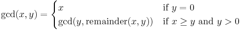
Greatest common divisor
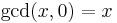
Another famous recursive function is the Euclidean algorithm, used to compute the greatest common divisor of two integers. Function definition:
| Pseudocode (recursive): |
|---|
function gcd is: input: integer x, integer y such that x >= y and y >= 0 |
Recurrence relation for greatest common divisor, where  expresses the remainder of
  :
:
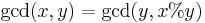
| Computing the recurrence relation for x = 27 and y = 9: |
|---|
gcd(27, 9)   = gcd(9, 27 % 9)
             = gcd(9, 0)
             = 9
|
| Computing the recurrence relation for x = 259 and y = 111: |
gcd(259, 111)   = gcd(111, 259 % 111)
                = gcd(111, 37)
                = gcd(37, 0)
                = 37
|
The recursive program above is tail-recursive; it is equivalent to an iterative algorithm, and the computation shown above shows the steps of evaluation that would be performed by a language that eliminates tail calls. Below is a version of the same algorithm using explicit iteration, suitable for a language that does not eliminate tail calls. By maintaining its state entirely in the variables x and y and using a looping construct, the program avoids making recursive calls and growing the call stack.
| Pseudocode (iterative): |
|---|
function gcd is: |
The iterative algorithm requires a temporary variable, and even given knowledge of the Euclidean algorithm it is more difficult to understand the process by simple inspection, although the two algorithms are very similar in their steps.
Towers of Hanoi
For a full discussion of this problem's description, history and solution see the main article or one of the many references.[5][6] Simply put the problem is this: given three pegs, one with a set of N disks of increasing size, determine the minimum (optimal) number of steps it takes to move all the disks from their initial position to another peg without placing a larger disk on top of a smaller one.
Function definition:
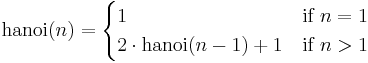
Recurrence relation for hanoi:

| Computing the recurrence relation for n = 4: |
|---|
hanoi(4)     = 2*hanoi(3) + 1
             = 2*(2*hanoi(2) + 1) + 1
             = 2*(2*(2*hanoi(1) + 1) + 1) + 1
             = 2*(2*(2*1 + 1) + 1) + 1
             = 2*(2*(3) + 1) + 1
             = 2*(7) + 1
             = 15
|
Example Implementations:
| Pseudocode (recursive): |
|---|
function hanoi is: |
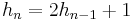
Although not all recursive functions have an explicit solution, the Tower of Hanoi sequence can be reduced to an explicit formula.[7]
| An explicit formula for Towers of Hanoi: |
|---|
h1 = 1   = 21 - 1
h2 = 3   = 22 - 1
h3 = 7   = 23 - 1
h4 = 15  = 24 - 1
h5 = 31  = 25 - 1
h6 = 63  = 26 - 1
h7 = 127 = 27 - 1
In general: hn = 2n - 1, for all n >= 1 |
Binary search
The binary search algorithm is a method of searching an ordered array for a single element by cutting the array in half with each pass. The trick is to pick a midpoint near the center of the array, compare the data at that point with the data being searched and then responding to one of three possible conditions: the data is found at the midpoint, the data at the midpoint is greater than the data being searched for, or the data at the midpoint is less than the data being searched for.
Recursion is used in this algorithm because with each pass a new array is created by cutting the old one in half. The binary search procedure is then called recursively, this time on the new (and smaller) array. Typically the array's size is adjusted by manipulating a beginning and ending index. The algorithm exhibits a logarithmic order of growth because it essentially divides the problem domain in half with each pass.
Example implementation of binary search in C:
 /*
  Call binary_search with proper initial conditions.

  INPUT:
    data is an array of integers SORTED in ASCENDING order,
    toFind is the integer to search for,
    count is the total number of elements in the array

  OUTPUT:
    result of binary_search

 */
 int search(int *data, int toFind, int count)
 {
    //  Start = 0 (beginning index)
    //  End = count - 1 (top index)
    return binary_search(data, toFind, 0, count-1);
 }

 /*
   Binary Search Algorithm.

   INPUT:
        data is a array of integers SORTED in ASCENDING order,
        toFind is the integer to search for,
        start is the minimum array index,
        end is the maximum array index
   OUTPUT:
        position of the integer toFind within array data,
        -1 if not found
 */
 int binary_search(int *data, int toFind, int start, int end)
 {
    //Get the midpoint.
    int mid = start + (end - start)/2;   //Integer division

    //Stop condition.
    if (start > end)
       return -1;
    else if (data[mid] == toFind)        //Found?
       return mid;
    else if (data[mid] > toFind)         //Data is greater than toFind, search lower half
       return binary_search(data, toFind, start, mid-1);
    else                                 //Data is less than toFind, search upper half
       return binary_search(data, toFind, mid+1, end);
 }
Recursive data structures (structural recursion)
An important application of recursion in computer science is in defining dynamic data structures such as Lists and Trees. Recursive data structures can dynamically grow to a theoretically infinite size in response to runtime requirements; in contrast, a static array's size requirements must be set at compile time.
"Recursive algorithms are particularly appropriate when the underlying problem or the data to be treated are defined in recursive terms." [8]
The examples in this section illustrate what is known as "structural recursion". This term refers to the fact that the recursive procedures are acting on data that is defined recursively.
As long as a programmer derives the template from a data definition, functions employ structural recursion. That is, the recursions in a function's body consume some immediate piece of a given compound value.[9]
Linked lists
Below is a simple definition of a linked list node. Notice especially how the node is defined in terms of itself. The "next" element of struct node is a pointer to another struct node, effectively creating a list type.
struct node
{
  int data;           // some integer data
  struct node *next;  // pointer to another struct node
};
Because the struct node data structure is defined recursively, procedures that operate on them can be implemented naturally as a recursive procedure. The list_print procedure defined below walks down the list until the list is empty (or NULL). For each node it prints the data element (an integer). In the C implementation, the list remains unchanged by the list_print procedure.
void list_print(struct node *list)
{
    if (list != NULL)               // base case
    {
       printf ("%d ", list->data);  // print integer data followed by a space
       list_print (list->next);     // recursive call on the next node
    }
}
Binary trees
Below is a simple definition for a binary tree node. Like the node for linked lists, it is defined in terms of itself, recursively. There are two self-referential pointers: left (pointing to the left sub-tree) and right (pointing to the right sub-tree).
struct node
{
  int data;            // some integer data
  struct node *left;   // pointer to the left subtree
  struct node *right;  // point to the right subtree
};
Operations on the tree can be implemented using recursion. Note that because there are two self-referencing pointers (left and right), tree operations may require two recursive calls:
// Test if tree_node contains i; return 1 if so, 0 if not.
int tree_contains(struct node *tree_node, int i) {
        if (tree_node == NULL)
                return 0;  // base case
        else if (tree_node->data == i)
                return 1;
        else
                return tree_contains(tree_node->left, i) || contains(tree_node->right, i);
}
At most two recursive calls will be made for any given call to tree_contains as defined above.
// Inorder traversal:
void tree_print(struct node *tree_node) {
        if (tree_node != NULL) {               // base case
                tree_print(tree_node->left);   // go left
                printf("%d ", tree_node->n);   // print the integer followed by a space
                tree_print(tree_node->right);  // go right
        }
}
The above example illustrates an in-order traversal of the binary tree. A Binary search tree is a special case of the binary tree where the data elements of each node are in order.
Filesystem traversal
Since the number of files in a filesystem may vary, recursion is the only practical way to traverse and thus enumerate its contents. Traversing a filesystem is very similar to that of tree traversal, therefore the concepts behind tree traversal are applicable to traversing a filesystem. More specifically, the code below would be an example of a preorder traversal of a filesystem.
import java.io.*;

public class FileSystem {

	public static void main (String [] args) {
		traverse ();
	}

	/**
	 * Obtains the filesystem roots
	 * Proceeds with the recurisve filesystem traversal
	 */
	private static void traverse () {
		File [] fs = File.listRoots ();
		for (int i = 0; i < fs.length; i++) {
			if (fs[i].isDirectory () && fs[i].canRead ()) {
				rtraverse (fs[i]);
			}
		}
	}

	/**
	 * Recursively traverse a given directory
	 *
	 * @param fd indicates the starting point of traversal
	 */
	private static void rtraverse (File fd) {
		File [] fss = fd.listFiles ();

		for (int i = 0; i < fss.length; i++) {
			System.out.println (fss[i]);
			if (fss[i].isDirectory () && fss[i].canRead ()) {
				rtraverse (fss[i]);
			}
		}
	}

}
This code blends the lines, at least somewhat, between recursion and iteration. It is, essentially, a recursive implementation, which is the best way to traverse a filesystem. It is also an example of direct and indirect recursion. "rtraverse" is purely a direct example; "traverse" is the indirect, which calls "rtraverse." This example needs no "base case" scenario due to the fact that there will always be some fixed number of files and/or directories in a given filesystem.
Recursion versus iteration
Expressive power
Most programming languages in use today allow the direct specification of recursive functions and procedures. When such a function is called, the program's runtime environment keeps track of the various instances of the function (often using a call stack, although other methods may be used). Every recursive function can be transformed into an iterative function by replacing recursive calls with iterative control constructs and simulating the call stack with a stack explicitly managed by the program.[10][11]
Conversely, all iterative functions and procedures that can be evaluated by a computer (see Turing completeness) can be expressed in terms of recursive functions; iterative control constructs such as while loops and do loops routinely are rewritten in recursive form in functional languages.[12][13] However, in practice this rewriting depends on tail call elimination, which is not a feature of all languages. C, Java, and Python are notable mainstream languages in which all function calls, including tail calls, cause stack allocation that would not occur with the use of looping constructs; in these languages, a working iterative program rewritten in recursive form may overflow the call stack.
Other considerations
In some programming languages, the stack space available to a thread is much less than the space available in the heap, and recursive algorithms tend to require more stack space than iterative algorithms. Consequently, these languages sometimes place a limit on the depth of recursion to avoid stack overflows. (Python is one such language.[14]) Note the caveat below regarding the special case of tail recursion.
There are some types of problems whose solutions are inherently recursive, because of prior state they need to track. One example is tree traversal; others include the Ackermann function, depth-first search, and divide-and-conquer algorithms such as Quicksort. All of these algorithms can be implemented iteratively with the help of an explicit stack, but the programmer effort involved in managing the stack, and the complexity of the resulting program, arguably outweigh any advantages of the iterative solution.
Tail-recursive functions
Tail-recursive functions are functions in which all recursive calls are tail calls and hence do not build up any deferred operations. For example, the gcd function (shown again below) is tail-recursive. In contrast, the factorial function (also below) is not tail-recursive; because its recursive call is not in tail position, it builds up deferred multiplication operations that must be performed after the final recursive call completes. With a compiler or interpreter that treats tail-recursive calls as jumps rather than function calls, a tail-recursive function such as gcd will execute using constant space. Thus the program is essentially iterative, equivalent to using imperative language control structures like the "for" and "while" loops.
| Tail recursion: | Augmenting recursion: |
|---|---|
//INPUT: Integers x, y such that x >= y and y > 0 int gcd(int x, int y) { if (y == 0) return x; else return gcd(y, x % y); } |
//INPUT: n is an Integer such that n >= 1 int fact(int n) { if (n == 1) return 1; else return n * fact(n - 1); } |
The significance of tail recursion is that when making a tail-recursive call, the caller's return position need not be saved on the call stack; when the recursive call returns, it will branch directly on the previously saved return position. Therefore, on compilers that support tail-recursion optimization, tail recursion saves both space and time.
Order of execution
In a recursive function, the position in which additional statements (i.e., statements other than the recursive call itself) are placed is important. In the simple case of a function calling itself only once, a statement placed before the recursive call will be executed first in the outermost stack frame, while a statement placed after the recursive call will be executed first in the innermost stack frame. Consider this example:
Function 1
void recursiveFunction(int num) {
   printf("%d\n", num);
   if (num < 4)
      recursiveFunction(num + 1);
}
Function 2 with swapped lines
void recursiveFunction(int num) {
   if (num < 4)
      recursiveFunction(num + 1);
   printf("%d\n", num);
}
Direct and indirect recursion
Most of the examples presented here demonstrate direct recursion, in which a function calls itself. Indirect recursion occurs when a function is called not by itself but by another function that it called (either directly or indirectly). "Chains" of three or more functions are possible; for example, function 1 calls function 2, function 2 calls function 3, and function 3 calls function 1 again.
See also
- Ackermann function
- Anonymous recursion
- Corecursion
- Functional programming
- Kleene–Rosser paradox
- McCarthy 91 function
- Memoization
- Mutual recursion
- μ-recursive function
- Primitive recursive function
- Recursion
- Sierpiński curve
- Takeuchi function
Notes and references
- ^ Graham, Ronald; Donald Knuth, Oren Patashnik (1990). Concrete Mathematics. Chapter 1: Recurrent Problems. http://www-cs-faculty.stanford.edu/~knuth/gkp.html.
- ^ Epp, Susanna (1995). Discrete Mathematics with Applications (2nd ed.). p. 427.
- ^ Wirth, Niklaus (1976). Algorithms + Data Structures = Programs. Prentice-Hall. p. 126.
- ^ Abelson, Harold; Gerald Jay Sussman (1996). Structure and Interpretation of Computer Programs. Section 1.2.2. http://mitpress.mit.edu/sicp/full-text/book/book-Z-H-11.html#%_sec_1.2.2.
- ^ Graham, Ronald; Donald Knuth, Oren Patashnik (1990). Concrete Mathematics. Chapter 1, Section 1.1: The Tower of Hanoi. http://www-cs-faculty.stanford.edu/~knuth/gkp.html.
- ^ Epp, Susanna (1995). Discrete Mathematics with Applications (2nd ed.). pp. 427–430: The Tower of Hanoi.
- ^ Epp, Susanna (1995). Discrete Mathematics with Applications (2nd ed.). pp. 447–448: An Explicit Formula for the Tower of Hanoi Sequence.
- ^ Wirth, Niklaus (1976). Algorithms + Data Structures = Programs. Prentice-Hall. p. 127.
- ^ Felleisen, Matthias (2002). "Developing Interactive Web Programs". In Jeuring, Johan. Advanced Functional Programming: 4th International School. Oxford, UK: Springer. p. 108
- ^ http://www.saasblogs.com/2006/09/15/how-to-rewrite-standard-recursion-through-a-state-stack-amp-iteration/
- ^ http://www.refactoring.com/catalog/replaceRecursionWithIteration.html
- ^ http://www.ccs.neu.edu/home/shivers/papers/loop.pdf
- ^ http://lambda-the-ultimate.org/node/1014
- ^ http://docs.python.org/library/sys.html
External links
- Harold Abelson and Gerald Sussman: "Structure and Interpretation Of Computer Programs"
- IBM DeveloperWorks: "Mastering Recursive Programming"
- David S. Touretzky: "Common Lisp: A Gentle Introduction to Symbolic Computation"
- Matthias Felleisen: "How To Design Programs: An Introduction to Computing and Programming"
- Duke University: "Big-Oh for Recursive Functions: Recurrence Relations"